
Welcome back! Today we will explore how you can leverage pandas to understand trends in time-series data quickly, with a particular focus on time-series methods like .resample, grouping by dates, and performing .rolling operations to smooth out the results. Along the way, I might grumble a bit (I’d like to think that the grey strands in my beard are from wisdom and not fighting with a computer), but I intend to give you some superpowers.
If you work with time series data, you will want to understand .resample, grouping, and .rolling, as they will make your life much easier.
The code below preserves that original environment and demonstrates the pandas concepts as they appeared in the original post.
Let’s start by picking a dataset that might be relevant considering recent news… bank failures.
Data Overview: FDIC BankFind Suite
In recent years, the banking sector in the United States has witnessed many financial institution failures, leading to substantial economic losses and systemic risks. The Federal Deposit Insurance Corporation (FDIC) bank failure data provides valuable insights into the underlying causes of these failures and helps develop effective risk management and regulatory compliance strategies. By exploring this data with the aid of the popular data analysis library, pandas, one can identify patterns and trends, prepare data for modeling, and visualize findings effectively.
BankFind Suite is a comprehensive database provided by the FDIC, which allows users to search for current and former FDIC-insured banking institutions based on name, FDIC certificate number, website, or location. This tool offers detailed information on an institution’s financial history and trends, enabling users to track the performance of individual institutions, groups of institutions, or the industry as a whole.
Let’s use the Bank Failure data to explore. I will download the data from 1934 to 2023 containing over 4000 entries.
import json
import pandas as pd
>>> df = pd.read_csv('bankfail.csv')
>>> df
    CERT    CHCLASS1    CITYST          COST    FAILDATE    FIN ID  NAME                    QBFASSET    QBFDEP      RESTYPE RESTYPE1    SAVR
0   15426.0 NM      ALMENA, KS      16806.0 10/23/2020  10538   4104    ALMENA STATE BANK           65733.0     64941.0     FAILURE PA      DIF
1   16748.0 NM      FORT WALTON BEACH, FL   7247.0  10/16/2020  10537   4103    FIRST CITY BANK OF FLORIDA      136566.0    133936.0    FAILURE PA      DIF
2   14361.0 NM      BARBOURSVILLE, WV   45913.0 4/3/2020    10536   4102    THE FIRST STATE BANK            151808.0    143102.0    FAILURE PA      DIF
3   18265.0 NM      ERICSON, NE     25293.0 2/14/2020   10535   4101    ERICSON STATE BANK          100879.0    95159.0     FAILURE PA      DIF
4   21111.0 N       NEWARK, NJ      1946.0  11/1/2019   10534   4100    CITY NATIONAL BANK OF NEW JERSEY    120574.0    111234.0    FAILURE PA      DIF
... ... ...     ...         ... ...     ... ... ...                 ...     ...     ... ...     ...
4099    NaN NM      LEWISPORT, KY       NaN 8/6/1934    0   137 BANK OF LEWISPORT           81.0        68.0        FAILURE PO      BIF
4100    NaN N       LIMA, MT        NaN 7/18/1934   0   135 FIRST NATIONAL BANK OF LIMA     91.0        42.0        FAILURE PO      BIF
4101    NaN NM      FLORENCE, IN        NaN 7/18/1934   0   136 FLORENCE DEPOSIT BANK           105.0       69.0        FAILURE PO      BIF
4102    NaN NM      EAST PEORIA, IL     NaN 5/28/1934   0   133 FON DU LAC STATE BANK           374.0       238.0       FAILURE PO      BIF
4103    NaN NM      PITTSBURGH, PA      NaN 4/19/1934   0   134 BANK OF AMERICA TRUST CO.       1435.0      1064.0      FAILURE PO      BIF
4104 rows × 13 columns
It looks like my CSV export loaded ok. However, the existing column names are a little annoying. I’m going to clean them up.
Here’s some code to rename the columns, create a city and state column, and convert the date column to a datetime type.
>>> colnames = {'CERT': 'cert',
...   'CHCLASS1': 'charter_class',
...    'CITYST': 'location',
...    'COST': 'estimated_loss',
...    'FAILDATE': 'effective_date',
...    'FIN': 'fin',
...    'ID': 'id',
...    'NAME': 'institution',
...    'QBFASSET': 'total_assets',
...    'QBFDEP': 'total_deposits',
...    'RESTYPE': 'resolution',
...    'RESTYPE1': 'transaction_type',
...    'SAVR': 'insurance_fund'}

>>> def tweak_bank(df):
...   return (df
...           .assign(FAILDATE=pd.to_datetime(df.FAILDATE, format='%m/%d/%Y'),
...                   city=df.CITYST.str.split(',').str[0],
...                   state=df.CITYST.str.split(',').str[1],
...                  )
...           .drop(columns=['CITYST'])
...           .rename(columns=colnames)
...          )

>>> bank = tweak_bank(df)
>>> bank
    cert    charter_class   estimated_loss  effective_date  fin id  institution             total_assets    total_deposits  resolution  transaction_type    insurance_fund  city            state
0   15426.0 NM      16806.0     2020-10-23  10538   4104    ALMENA STATE BANK           65733.0     64941.0     FAILURE     PA          DIF     ALMENA          KS
1   16748.0 NM      7247.0      2020-10-16  10537   4103    FIRST CITY BANK OF FLORIDA      136566.0    133936.0    FAILURE     PA          DIF     FORT WALTON BEACH   FL
2   14361.0 NM      45913.0     2020-04-03  10536   4102    THE FIRST STATE BANK            151808.0    143102.0    FAILURE     PA          DIF     BARBOURSVILLE       WV
3   18265.0 NM      25293.0     2020-02-14  10535   4101    ERICSON STATE BANK          100879.0    95159.0     FAILURE     PA          DIF     ERICSON         NE
4   21111.0 N       1946.0      2019-11-01  10534   4100    CITY NATIONAL BANK OF NEW JERSEY    120574.0    111234.0    FAILURE     PA          DIF     NEWARK          NJ
... ... ...     ...     ...     ... ... ...                 ...     ...     ...     ...         ...     ...         ...
4099    NaN NM      NaN     1934-08-06  0   137 BANK OF LEWISPORT           81.0        68.0        FAILURE     PO          BIF     LEWISPORT       KY
4100    NaN N       NaN     1934-07-18  0   135 FIRST NATIONAL BANK OF LIMA     91.0        42.0        FAILURE     PO          BIF     LIMA            MT
4101    NaN NM      NaN     1934-07-18  0   136 FLORENCE DEPOSIT BANK           105.0       69.0        FAILURE     PO          BIF     FLORENCE        IN
4102    NaN NM      NaN     1934-05-28  0   133 FON DU LAC STATE BANK           374.0       238.0       FAILURE     PO          BIF     EAST PEORIA     IL
4103    NaN NM      NaN     1934-04-19  0   134 BANK OF AMERICA TRUST CO.       1435.0      1064.0      FAILURE     PO          BIF     PITTSBURGH      PA
4104 rows × 14 columns
Not bad. This is going to be great data for learning .resample, .groupby, and .rolling.
Data Dictionary
Here is the description of the columns for those (like me) who aren’t subject matter experts. (All descriptions taken from here.)
- cert – Certificate number assigned by FDIC to identify the institution
- charter_class – The FDIC assigns classification codes indicating an institution’s charter type (commercial bank, savings bank, or savings association), its chartering agent (state or federal government), its Federal Reserve membership status (member or nonmember), and its primary federal regulator (state-chartered institutions are subject to both federal and state supervision). These codes are:
- N National chartered commercial bank supervised by the Office of the Comptroller of the
- SM State charter Fed member commercial bank supervised by the Federal Reserve
- NM State charter Fed nonmember commercial bank supervised by the FDIC
- SA State or federal charter savings association supervised by the Office of Thrift Supervision or Office of the Comptroller of the Currency
- SB State charter savings bank supervised by the FDIC
- estimated_loss – the difference between the amount disbursed from the Deposit Insurance Fund (DIF) to cover obligations to insured depositors and the amount estimated to be ultimately recovered from the liquidation of the receivership estate. Estimated losses reflect unpaid principal amounts deemed unrecoverable and do not reflect interest that may be due on the DIF’s administrative or subrogated claims should its principal be repaid in full.
- effective_date – date of failure.
- fin – Financial institute number. Another unique identifier.
- id – Institution directory number
- name – Legal name of the institution.
- total_assets – The Total assets owned by the institution, including cash, loans, securities, bank premises, and other assets as of the last Call Report or Thrift Financial Report.
- total_deposits – Total including demand deposits, money market deposits, other savings deposits, time deposits and deposits in foreign offices as of the last Call Report.
- resolution – Failure stature. Failure or assistance by merging with other institution.
- transaction_type – Resolution type. Cat 1 – Institution’s charter survives. Cat 2 – Charter terminated. Cat 3 – Payout:
- A/A – Cat1. (Assistance Transactions). Assistance was provided to the acquirer, who purchased the entire institution.
- REP – Cat1. Re-privatization, management takeover with or without assistance at takeover, followed by a sale with or without additional assistance.
- P&A – Cat2. Purchase and Assumption, where some or all of the deposits, certain other liabilities, and a portion of the assets (sometimes all of the assets) were sold to an acquirer. It was not determined if all the deposits (PA) or only the insured deposits (PI) were assumed.
- PA – Cat2. Purchase and Assumption, where the insured and uninsured deposits, certain other liabilities, and a portion of the assets were sold to an acquirer.
- PI – Cat2. Purchase and Assumption of the insured deposits only, where the traditional P&A was modified so that the acquiring institution assumed only the insured deposits.
- IDT – Cat2. Insured deposit Transfer, where the acquiring institution served as a paying agent for the insurer, established accounts on their books for depositors and often acquired some assets as well.
- ABT – Cat2. Asset-backed transfer, an FSLIC transaction that is very similar to an IDT.
- MGR – Cat2.An institution where FSLIC took over management and generally provided financial assistance. FSLIC closed down before the institution was sold. transactions
- PO – Cat3 – Payout, where the insurer paid the depositors directly and placed the assets in a liquidating receivership.
- insurance_fund – Insurance fund.
Counts of failures by year
Let’s use pandas to find the count of failures by year.
When I hear the words “by year,” I immediately think we need to group this data by year. This is like one of those word math problems that everyone hated in junior high until they understood how to convert the words to math. The same thing happens here. When your boss tells you they want “failures by year,” you should think, “I’m going to use the year column in the pandas .groupby method.”
In this case, we don't have a year column. But due to the magic of datetime columns, we can access the year through the .dt accessor.
>>> bank.effective_date
0      2020-10-23
1      2020-10-16
2      2020-04-03
3      2020-02-14
4      2019-11-01
          ...
4099   1934-08-06
4100   1934-07-18
4101   1934-07-18
4102   1934-05-28
4103   1934-04-19
Name: effective_date, Length: 4104, dtype: datetime64[ns]
>>> (bank
...  .groupby(bank.effective_date.dt.year)
...  .size()
... )
effective_date
1934     9
1935    25
1936    69
1937    75
1938    74
        ..
2015     8
2016     5
2017     8
2019     4
2020     4
Length: 84, dtype: int64
This is ok. I would prefer a visualization to this table of data. Let’s try a bar chart.
(bank
 .groupby(bank.effective_date.dt.year)
 .size()
 .plot.bar()
)
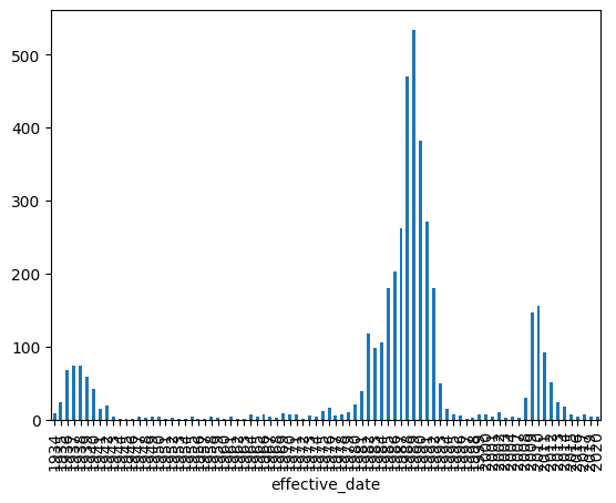
This is a start, but the x-axis is not happy. Just be aware that if you intend on making bar plots with pandas, it converts the index to categories. In this case, the dates are converted to strings. This makes me sad, but not every library is perfect.
https://github.com/pandas-dev/pandas/issues/17001
Let’s try and make a line plot instead.
(bank
 .groupby(bank.effective_date.dt.year)
 .size()
 .plot()
)
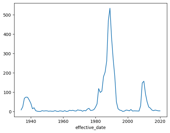
This looks good. Line plots in pandas (unlike bar plots) respect dates in the index.
Now let’s jump into grouping functionality that is time-series specific.
Using Offset Aliases with Pandas Resample
Hidden away in the pandas documentation is a mention of offset aliases. (Sadly, these are not accessible from the docstrings inside of Jupyter, which is one lament I have with pandas otherwise excellent documentation).
You can find them here, or documented in my book, Effective Pandas.
In short, Y, Q, M, W, and D mean year, quarter, month, week, and day respectively. If you memorize these single-letter shortcuts, the .resample method, or the pd.Grouper class, you can quickly aggregate date information by different time intervals.
Let's try and view failures by month using the .resample method. Pandas resampling is powerful because it lets you convert time-series data with one time interval into time-series data with different time intervals. You can upsample so you have more rows over shorter intervals, or downsample so you have fewer rows over longer intervals. The key to using this method is sticking a date column into the index and then calling .resample instead of .groupby:
>>> (bank
...  .set_index('effective_date')
...  .resample('M')
...  .size()
... )
effective_date
1934-04-30    1
1934-05-31    1
1934-07-31    2
1934-08-31    1
1934-09-30    1
             ..
2019-10-31    2
2019-11-30    1
2020-02-29    1
2020-04-30    1
2020-10-31    2
Length: 540, dtype: int64
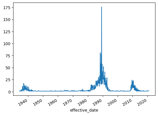
Notice the index in the resulting Series. Each entry ends on the last day of the month. This is because we passed the M (month) offset alias into the .resample method.
I generally plot this by chaining on a call to .plot. This will plot the date on the x-axis and draw the values on the y-axis.
(bank
 .set_index('effective_date')
 .resample('M')
 .size()
 .plot()
)
Smoothing By Rougher Aggregations Using Pandas Resample
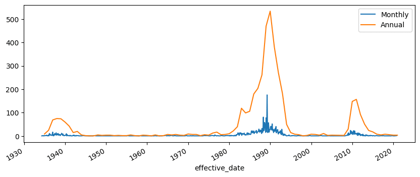
Let’s try something a little fancier. We will make a function that plots the monthly failures (which we already saw was bumpy) and then plot the yearly aggregation on top.
I'll use the .pipe method to refactor the plotting logic into a single function.
>>> import matplotlib.pyplot as plt
>>> fig, ax = plt.subplots(figsize=(10,4))
>>> def plot_monthly_and_yearly(df, ax):
...     (df
...       .resample('M')
...       .size()
...       .plot(ax=ax, label='Monthly')
...     )
...     (df
...       .resample('Y')
...       .size()
...       .plot(ax=ax, label='Annual')
...     )
...     ax.legend()
...     return df

>>> (bank
...  .set_index('effective_date')
...  .pipe(plot_monthly_and_yearly, ax=ax)
... )
        cert    charter_class   estimated_loss  fin id  institution             total_assets    total_deposits  resolution  transaction_type    insurance_fund  city            state
effective_date
2020-10-23  15426.0 NM      16806.0     10538   4104    ALMENA STATE BANK           65733.0     64941       FAILURE     PA          DIF     ALMENA          KS
2020-10-16  16748.0 NM      7247.0      10537   4103    FIRST CITY BANK OF FLORIDA      136566.0    133936      FAILURE     PA          DIF     FORT WALTON BEACH   FL
2020-04-03  14361.0 NM      45913.0     10536   4102    THE FIRST STATE BANK            151808.0    143102      FAILURE     PA          DIF     BARBOURSVILLE       WV
2020-02-14  18265.0 NM      25293.0     10535   4101    ERICSON STATE BANK          100879.0    95159       FAILURE     PA          DIF     ERICSON         NE
2019-11-01  21111.0 N       1946.0      10534   4100    CITY NATIONAL BANK OF NEW JERSEY    120574.0    111234      FAILURE     PA          DIF     NEWARK          NJ
...     ... ...     ...     ... ... ...                 ...     ...     ...     ...         ...     ...         ...
1934-08-06  NaN NM      NaN     0   137 BANK OF LEWISPORT           81.0        68      FAILURE     PO          BIF     LEWISPORT       KY
1934-07-18  NaN N       NaN     0   135 FIRST NATIONAL BANK OF LIMA     91.0        42      FAILURE     PO          BIF     LIMA            MT
1934-07-18  NaN NM      NaN     0   136 FLORENCE DEPOSIT BANK           105.0       69      FAILURE     PO          BIF     FLORENCE        IN
1934-05-28  NaN NM      NaN     0   133 FON DU LAC STATE BANK           374.0       238     FAILURE     PO          BIF     EAST PEORIA     IL
1934-04-19  NaN NM      NaN     0   134 BANK OF AMERICA TRUST CO.       1435.0      1064        FAILURE     PO          BIF     PITTSBURGH      PA
4104 rows x 13 columns
Resolution Type Over Time
I want to talk about one more feature of pandas: the pd.Grouper class. I use this class to group by different frequencies of a date column without having to stick the date in the index and call .resample. You might ask, why?
The .resample method only allows us to have a single grouping. If you have played around with .groupby, then you know that you can provide multiple columns or series to .groupby. In this example, let's assume this word problem:
What are the counts of the different resolution types by month?
This is a little tricky. We have “by month,” so we want to group by month, but we also really have “size by resolution type by month.”
A first stab might look like this:
>>> (bank
...  .groupby([bank.effective_date.dt.month, 'resolution'])
...  .size()
... )
effective_date  resolution
1               ASSISTANCE     22
                FAILURE       274
2               ASSISTANCE     26
                FAILURE       302
3               ASSISTANCE     32
                FAILURE       443
4               ASSISTANCE     87
                FAILURE       328
5               ASSISTANCE     30
                FAILURE       283
6               ASSISTANCE     28
                FAILURE       298
7               ASSISTANCE     48
                FAILURE       359
8               ASSISTANCE     62
                FAILURE       280
9               ASSISTANCE     57
                FAILURE       219
10              ASSISTANCE     47
                FAILURE       284
11              ASSISTANCE     30
                FAILURE       212
12              ASSISTANCE    110
                FAILURE       243
dtype: int64
This sort of works if we want to know how many banks failed in December. But we want monthly data over time. Because we also want to group by resolution, we can't use the .resample method. This is where pd.Grouper comes in.
We provide the name of a datetime column and a frequency (this is that offset alias that we talked about above). The code looks like this:
>>> (bank
...  .groupby([pd.Grouper(key='effective_date', freq='M'),
...            'resolution'])
...  .size()
... )
effective_date  resolution
1934-04-30      FAILURE       1
1934-05-31      FAILURE       1
1934-07-31      FAILURE       2
1934-08-31      FAILURE       1
1934-09-30      FAILURE       1
                             ..
2019-10-31      FAILURE       2
2019-11-30      FAILURE       1
2020-02-29      FAILURE       1
2020-04-30      FAILURE       1
2020-10-31      FAILURE       2
Length: 635, dtype: int64
By now, you know that I want to plot this. However, tacking on .plot is unsatisfying as we have a hierarchical index and this sticks both date and resolution as a tuple on the x-axis:
(bank
 .groupby([pd.Grouper(key='effective_date', freq='M'),
           'resolution'])
 .size()
 .plot()
)
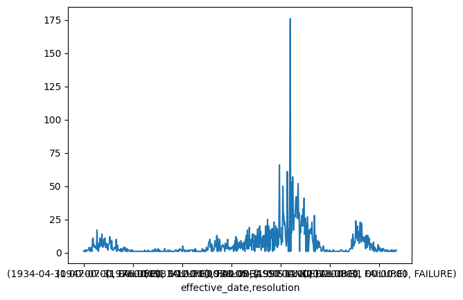
What I want to do instead is unstack the innermost index, the resolution index. The .unstack method will pull out the inner index by default and stick it up into the columns. Now we have monthly dates in the index and a column for each resolution type.
>>> (bank
...  .groupby([pd.Grouper(key='effective_date', freq='M'),
...            'resolution'])
...  .size()
...  .unstack(level=1)
... )
        __reduced___ASSISTANCE  __reduced___FAILURE
effective_date
1934-04-30  NaN         1
1934-05-31  NaN         1
1934-07-31  NaN         2
1934-08-31  NaN         1
1934-09-30  NaN         1
...     ...         ...
2019-10-31  NaN         2
2019-11-30  NaN         1
2020-02-29  NaN         1
2020-04-30  NaN         1
2020-10-31  NaN         2
540 rows x 2 columns
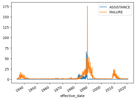
If we plot this, we will get a line for each resolution type over time. It looks like the FAILURE resolution is much more common since 1989.
def fix_cols(name):
    return name.replace('__reduced___', '')

(bank
 .groupby([pd.Grouper(key='effective_date', freq='M'),
           'resolution'])
 .size()
 .unstack(level=1)
 .fillna(0)
 .rename(columns=fix_cols)
 .plot()
)
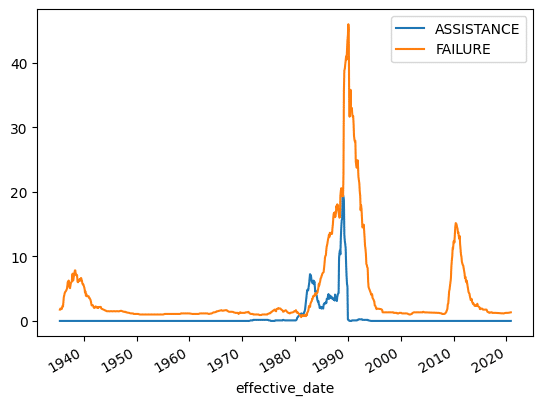
Let’s do a 12-month rolling average to smooth this out a bit.
(bank
 .groupby([pd.Grouper(key='effective_date', freq='M'),
           'resolution'])
 .size()
 .unstack(level=1)
 .rename(columns=fix_cols)
 .fillna(0)
 .rolling(12)
 .mean()
 .plot()
)
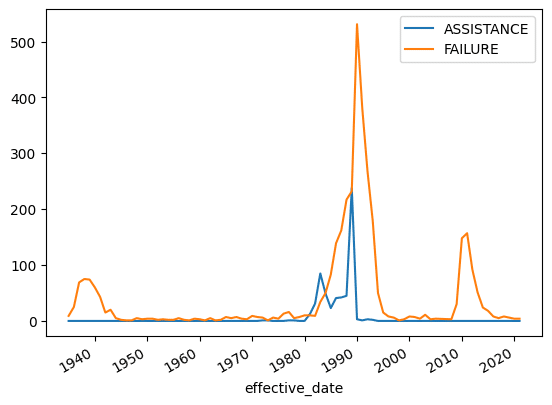
Below I plot the yearly resolution size. Again, you can see that the basic shape is the same, but the yearly rolling average tells a better story.
(bank
 .groupby([pd.Grouper(key='effective_date', freq='Y'),
           'resolution'])
 .size()
 .unstack(level=1)
 .rename(columns=fix_cols)
 .fillna(0)
 .plot()
)
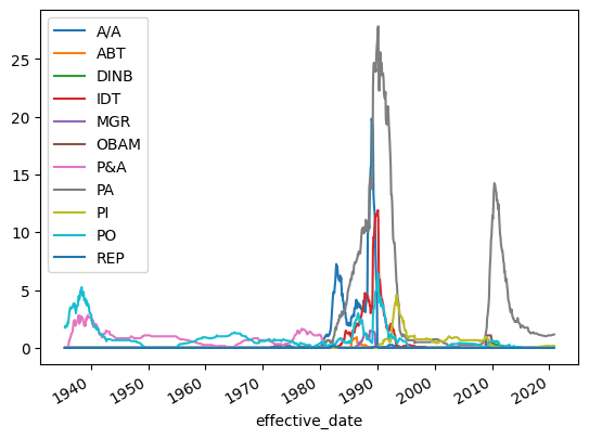
And finally, let’s look at the 12-month rolling average by resolution type.
(bank
 .groupby([pd.Grouper(key='effective_date', freq='M'),
           'transaction_type'])
 .size()
 .unstack(level=1)
 .rename(columns=fix_cols)
 .fillna(0)
 .rolling(12)
 .mean()
 .plot()
)
Now You Have Pandas Resample, Groupby, and Rolling Superpowers
I hope that this blog post exposed you to the powerful time-series functionality in pandas, particularly .resample, .groupby, and .rolling.
Folks often ask me why I use pandas to manipulate my data. Could I do this in SQL? Yes… probably. But I’ve written enough SQL in my life to know that it wouldn’t be fun for me.